Research highlights 2021
The articles below are based on scientific articles and reflect our different research areas. They were originally published in the Bolin Centre’s annual report 2021.

RA1 | Research highlights
Observation-based Climate models selected with support in observational data projects Arctic ice-free summers from 2035 onwards
The retreat of Arctic sea ice is one of the most striking consequences of global warming and has strong implications for local and remote climate, biosphere and society.
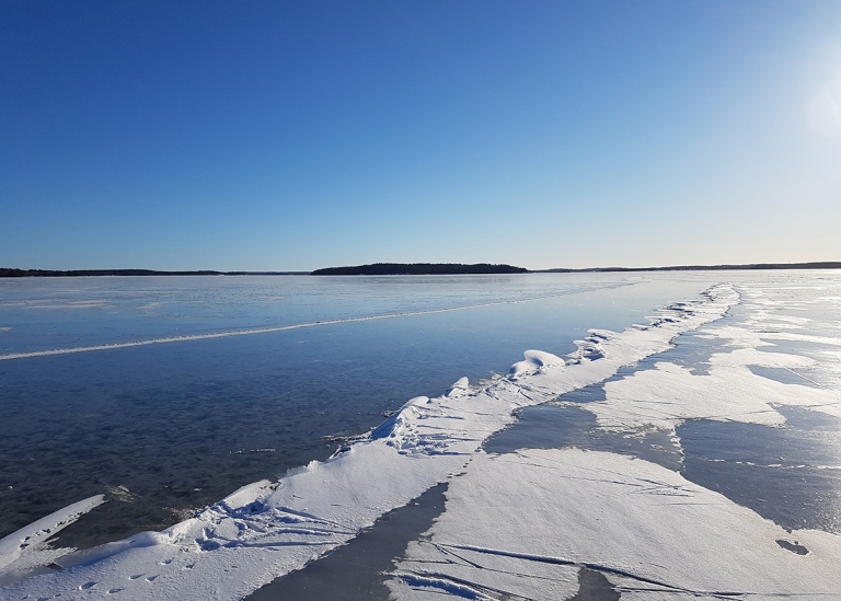
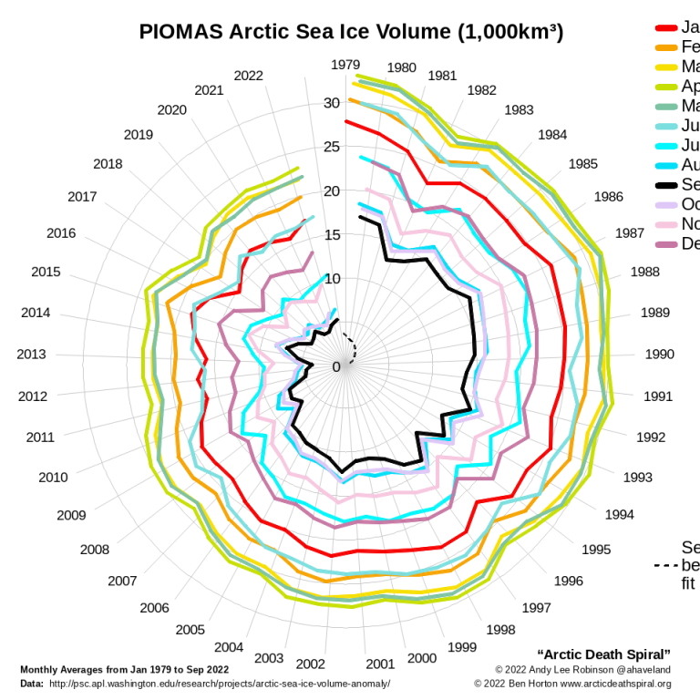
The total area of the Arctic Ocean covered by sea ice has decreased by about 2 million km2 in the past 40 years of satellite observations, with more pronounced loss in the summer. As sea ice has also thinned by 1.5–2 m in the central Arctic, the total Arctic sea-ice volume has decreased as well, from around 15,000 km3 to 5,000 km3 in summer (in winter from around 30,000km3 to slightly above 20,000 km3). The current Arctic sea-ice losses are strongly connected to rising global temperatures and thus to the increased greenhouse gas emissions into the atmosphere.
Our best tool to investigate how the Arctic sea ice will develop in the future are climate models coupling the atmosphere, ocean and land. The latest generation of climate models, which has been contributed to the 6th phase of the Coupled Model Intercomparison Project (CMIP6) and fed into the Intergovernmental Panel on Climate Change (IPCC) Assessment Report 6, performed climate mod-el projections following different future greenhouse gas emission and land-use scenarios until year 2100. While these latest models are generally better representing the observed changes of Arctic sea ice compared to earlier model generations, a number of individual models still substantially over- or underestimate the observed sea ice conditions and trends. Thus, just calculating the average over all the models might not provide the best estimate for future sea ice development. On the other hand, it is not given that a model that simulates todays ice conditions best is also best to simulate future conditions, which means that selecting only one or very few models might lead to an overconfidence in the results.
Our study selects thus the half of all climate models that best represents the observed present Arctic sea-ice area and thickness, their trends, and northward ocean heat transport into the Arctic, as the latter is a major driver of recent sea-ice loss. Thereby, we exclude those models, which deviate strongly from the observed conditions and which are thus likely not well suited to reliable project the future sea ice, but we still include a variety of models allowing for different outcomes based on the different models.

We find that the sea-ice loss over this century is larger using our different model selection criteria compared to the average over all models without model selection. In particular, we find that sum-mer ice-free Arctic conditions could occur as early as year 2035 in the selection case, compared to around 2060 in the no-selection case following a high-emission scenario. Even in a low-emission scenario, the selection of models based on their performance in the past leads to a much stronger sea ice reduction compared to averaging over all models, and an almost 50% probability for a total summer ice loss in the 21st century. Our results highlight a potential underestimation of the future Arctic sea-ice loss when including all models that contributing to CMIP6.
The article was published in Communications Earth & Environment and can be found here:
Observation-based selection of climate models projects Arctic ice-free summers around 2035
RA2 | Research highlights
New insights into ultrafine aerosols in the high Arctic
One major uncertainty in future climate projections concerns how aerosol particles impact cloud properties and distribution. Pristine summer Arctic low-level clouds contain low numbers of activated aerosol particles. Therefore, these clouds are often optically thin and have fewer but larger droplets compared to other regions. Combined with the semi-permanent ice cover, small changes in either the number of natural aerosol particles or the ice cover are very important to the heat transfer to the ice and the subsequent ice-melt. A team of researchers from different departments took a closer look at the aerosol formation process in this climate-critical and changing region, and found a surprising result.
Clouds are an important part of the Earth’s climate system. They play a role in controlling how much energy passes from the sun to Earth’s surface, and from the surface back out into the space. Aerosols – small, invisible particles in the air – acts as seeds onto which water can condense to form cloud droplets. The high Arctic region, near the North Pole, is a unique environment, with median daily very low aerosol concentrations ranging typically between 15 and 30 percm3, and occasionally below 1 per cm3. These conditions impact the formation of clouds and their energy trapping and releasing properties. For large parts of the year, the surface reflectivity is as high as, or higher than, the cloud albedo, and longwave radiation processes dominate, thus constituting a net warming effect. During the most intense summer ice melt, surface reflectivity is reduced when melting sea ice opens up dark ocean surfaces and melt ponds form on the ice. Low-level clouds may therefore cool the surface for a short time period in summer.
One key question is which sources may contribute to the aerosol over the central Arctic Ocean. It has been shown that the concentration of transported continental aerosols, influenced by man-made activities, and aerosol precursors are extremely low over the pack ice. The absence of strong winds over the relatively small area of open water, 10–30 percent, in the pack ice has been observed also to result in a weak local source of primary sea spray aerosol. In fact, aerosol concentrations in the summer time high Arctic are sometimes low enough to prevent cloud formation. This means that even if the local natural aerosol source is weak, it can have a significant impact on cloudiness, surface temperature, and ice melt.
Previous Stockholm University coordinated Arctic studies in the years of 1991, 1996, 2001 and 2008, on the Swedish icebreaker Oden, have been successful in demonstrating that local emissions of marine biota can form clouds. Near-surface aerosols, as well as low-level cloud and fog droplets, contained the same type of organic material, as found in the leads (open water between ice floes) in support of a local or regional aerosol source within the pack ice.
The established weak lead source of particles could however not explain the simultaneously observed near-surface airborne aerosol concentrations.
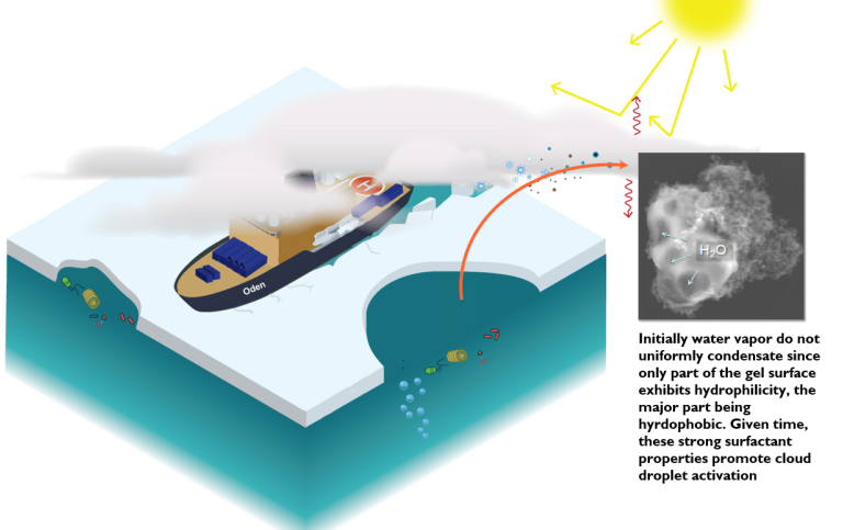
Nonetheless, the appearance of high concentration of ultrafine particles (smaller than 100 nm in diameter, also called the Aitken mode), under certain conditions (sunny with intermittent fog and light winds, melting of the fringes or during early refreezing of the leads), strongly suggests substantial particle sources in the innermost Arctic. To explain this, it has been speculated that the marine biota, which behaved similar to marine polymer gels (3D cross-linked networks of poly saccharides stabilized by Ca2+ bonds and/or hydrophobic forces), once airborne, would disintegrate and generate progressively smaller particles.
On the most recent expedition in 2018, an Aitken mode event presented itself. For the first time, researchers managed to measure the chemical composition of the ultrafine particles over time. They found that these very tiny particles indeed contained polysaccharides. To their surprise, it also seemed as if large numbers of particles were formed from the breakup of larger composite particles, which corroborates earlier speculations. At this stage the mechanism for subsequent breakup of gel aggregates in the atmosphere is difficult to assess and remains an open research question.
What are the implications of the results? How can they be used?
“One overall implication of these new results is that they may explain why only a few percent of the observed airborne total particle number variability was explained by the direct measurements of particle number fluxes and as such strongly suggest substantial particle sources, behaving similar to marine gels, in the innermost Arctic”, says Caroline Leck, one of the researchers in the study. The presence of marine gel-particles in the atmosphere were first discovered in the year of 1996.
Furthermore, the suggested a hydrophobic character for the central Arctic Aitken-mode aerosols would in turn impede water uptake and suppress cloud activation. As such, it seems that very high-water supersaturations, about four times higher than for larger sized and more water-soluble particles, would be required in order for the Aitken mode particles to be activated. Based on a large-eddy simulation (LES) study it seems possible that such high-water supersaturations occur where small total droplet number concentrations are present such that excess water vapor is not depleted by larger particles and helps sustain the cloud even when the Aitken particles have low hygroscopicity.

What could be the next natural step in this area of research?
“The Arctic is a region to which one must return again and again in order to succeed. In the end, most often the success is a matter of happenstance.”
The study was conducted by several Bolin Centre members across different departments; Linn Karlsson, Matthew Salter, and Paul Ziegler at the Department of Environmental Science, and Caroline Leck at the Department of Meteorology. First author was Mike Lawler, Department of Earth System Science at the University of California.
The article "New Insights Into the Composition and Origins of Ultrafine Aerosol in the Summertime High Arctic" was first published on 25 October 2021 in Geophysical Research Letters. The article can be accessed here:
New Insights Into the Composition and Origins of Ultrafine Aerosol in the Summertime High Arctic
This work was supported by the United States’ National Science Foundation Arctic Natural Sciences program, Swedish Research Council, the Bolin Centre for Climate Research (RA2), Swiss National Science Foundation, the Swiss Polar Institute, the BNP Paribas Swiss Foundation, the Knut and Alice Wallenberg Foundation within the ACAS project (Arctic Climate Across Scales), and Swedish Polar Research.
RA3 | Research highlights

Online seminar series – Perspectives of Hydrology and Water Resources
Research Area 3 has focused on an online seminar series called Perspectives of Hydrology and water resources. Renowned researchers from around the world were invited to present. In 2021, four webinars were announced.
The first presenter in the seminar series was Prof. Jay Famiglietti from the University of Saskatchewan, Canada, who gave a presentation titled:
Emerging Threats to Global Water Security as Viewed from Space
The evolving water cycle of the 21st century is proving to be stronger and more variable, resulting in broad swaths of mid-latitude drying, accelerated by the depletion of the world’s major groundwater aquifers. A well-defined geography of freshwater ‘haves’ and ‘have-nots’ is clearly emerging. What does water sustainability mean under such dynamic climate and hydrologic conditions, in particular when coupled with future projections of population growth? How will water managers cope with these new normals, and how will food and energy production be impacted?
Jay reviewed what nearly two decades of satellite research tells us about emerging threats to water security. He shared his personal experiences with science communication and water diplomacy, and encouraged the next generation of water scientists to seek out transdisciplinary experiences as part of their graduate and postgraduate training.
Jay is also a member of the Bolin Centre’s External Science Advisory Group.
Climate scientist Lukas Gudmundsson at the Institute of Atmospheric and Climate Science, ETH Zurich, Switzerland, presented under the heading:
Detecting and attributing global change in terrestrial water systems
One of the key concerns with anthropogenic climate change are its effects on the terrestrial water cycle. Model projections indicate that anthropogenic climate change can affect regional water availability and may trigger more floods and droughts. While there is mounting evidence showing human impacts in the atmospheric part of the water cycle, the limited availability of relevant observations has so far prevented an unambiguous detection and attribution of anthropogenic climate change in terrestrial water resources and hydrological extremes.
Recent advances in mobilizing large quantities of river flow time series around the globe and breakthroughs in data-driven reconstructions of essential freshwater variables using machine learning now allow for an unprecedented assessment of global hydrological change. Causal drivers of observed change are investigated using climate change detection and attribution methods, that ingest both observational information and model-based evidence. The analysis allows to conclude that it is very likely that anthropogenic climate change is already impacting water resources and hydrological extremes at the global scale.
Dr. Fabrice Papa at the Institut de Recherche pour le Développement in France, presented:
The variability of water storage and fluxes over large tropical river basins from multi-satellite observations and their impacts on the land-ocean continuum
Terrestrial waters, despite being less than one percent of the total amount of water on Earth’s ice-free land are essential for life and human environment. They play a primary role in the global water and carbon cycles, with significant impacts on climate variability. A better characterization of their distribution and dynamic over the whole globe is therefore of highest priority, including for the management of water resources. However, despite their importance, basic questions are still open, such as: what are the spatio-temporal variations of the fluxes and storages of continental freshwater across scales and how do they interact with climate and the anthropogenic pressure? Those questions are specifically important for the Tropics which are now facing growing demands for freshwater availability.
During the seminar, Fabrice discussed different observation techniques to quantify the freshwater variations in different parts of the Earth.
Marc F.P. Bierkensat the Department of Physical Geography, Utrecht University in the Netherlands, presented:
Advances in Modelling Global Hydrology and Water Resources under Change
This seminar reviews the current state of global hydrological and water resources modelling under change, discusses past and recent developments, and extrapolates these to future challenges and directions. It starts with describing the history of global hydrological model development in three established domains: atmospheric modelling, global water resources assessment and dynamic vegetation modelling. Next, a genealogy of global hydrological models is given. Thereafter, recent efforts to connect model components from different domains are reviewed with special reference to multi-sectoral inter-comparison projects. Also, new domains of application are identified where global hydrology is now starting to become an integral part of the analyses.
Marc ended the seminar with a short overview of recent and future work on global hydrology and water resources in his own group on three related subjects: very-high resolution global modelling of surface and groundwater hydrology; including surface water quality and groundwater salinity; the global limits of groundwater use.

Useful tool to help water scientists keep together
What was the aim of this online series and how did it turn out?
We asked RA3 leader Fernando Jaramillo.
“It has been difficult for us to interact during the pandemic. It has also been challenging to invite renowned scientists to the Bolin Centre to describe their latest scientific research concerning water. The online series on Perspectives of Hydrology and Water Resources aimed to bring these important scientists to our researchers’ homes. We had a high attendance rate, in some cases above 50 participants, with active discussion and interesting questions from the public. It was definitely a useful tool to help water scientists keep together within the Bolin Centre” says RA3 leader Fernando Jaramillo.
RA4 | Research highlights
High methane emissions from shallow-water northern temperate coastal habitats partially offset the coastal carbon sink
The human atmospheric warming from methane is second after only that of carbon dioxide. Since the beginning of the industrialisation the global methane atmospheric inventory has increased by 150 percent due to agricultural, industrial, and natural emissions. Because of its short half-life of 12 years in the atmosphere, methane is established as the most important short-term climate forcer with the greatest potential for climate mitigation over the next decades. Understanding and controlling methane emissions is therefore of key importance for near-term climate mitigation efforts. In order to achieve this goal, it is important to pinpoint the key emitters and to understand the regulating biogeochemical dynamics under which they operate.
Assessing the quantitative feedbacks of anthropogenic change on naturally occurring processes poses significant challenges. Depending on how the emissions are apportioned to their putative different sources, significant discrepancies arise in the emission budgets. If bottom-up approaches are used – summing up the emissions from putative sources, significantly larger emissions are calculated than when top-down approaches are used, i.e., when back-calculating from atmospheric measurements to their putative sources using air mass trajectories. The correct apportionment therefore involves several challenges:
- what specific area and environment is the emitter and at what magnitude is methane emitted?
- how will the area and environment change in the future?
- where and what effective nature-based solutions may be used to mitigate carbon emissions?
The formation and emission of methane occurs largely through microbial activity in soils and sediment and is directly related to the occurrence of organic-rich habitats with low levels of oxygen. Here, large amounts of organic matter are fixed photosynthetically or have accumulated historically. Aquatic ecosystems comprise about 50 percent of the natural global methane emissions. Northern temperate shallow-water coastal wetlands and seagrass beds can be such highly productive systems, but have strong temporal and spatial variability in methane emissions. While freshwater environments have long been in the focus as methane sources, northern coastal wetlands, seagrass beds and macroalgal beds have now come into the focus as, so far, underestimated methane sources. Coincidently, these ecosystems, some of which are the most productive ecosystems on Earth, have also been the targets of blue carbon efforts to mitigate carbon accumulation through natural carbon storage. Significant methane emissions from them would significantly offset their carbon mitigation potential.
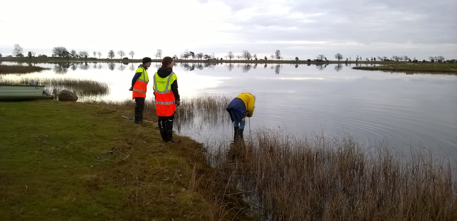
A team of Bolin Centre researchers joined forces with scientists from the Baltic Sea Research Centre at Stockholm University and initiated a long-term investigation to establish the temporal variability of methane emissions from high latitude organic-rich marine coastal environments. Specifically, they wanted to address the scaling problem for inshore coastal ecosystems and to quantify the methane emissions in these habitats.
Directly capturing the spatial and temporal variability of emissions simultaneously by bottom-up scaling is not practically possible. Instead, one has to rely on continuous measurements in a few selected key habitats, and combine these with discrete measurements at many different localities and times. These measurements can then be used to calibrate widely available environmental monitoring data, and to extrapolate the measured emissions.
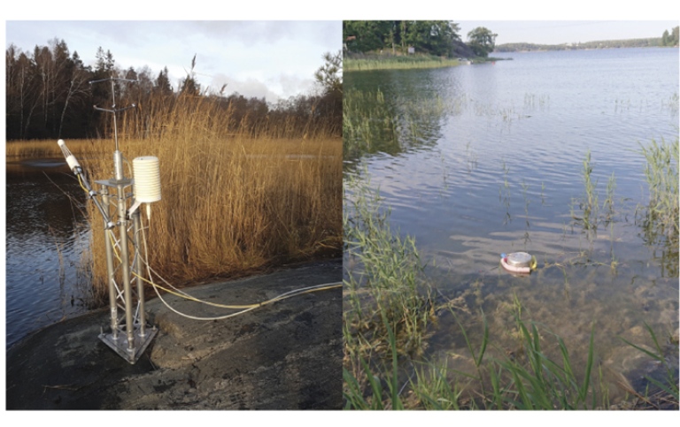
In an effort to scale the observed emissions over a large area of the Baltic coast, the researchers used a small eddy correlation tower and conducted high-frequency methane and carbon dioxide analyses with a laser spectrometer at the tower. These data were combined with a large array of flux measurements, diverse instrumental arrays and different techniques of field and laboratory analyses in order to quantify methane fluxes throughout the year and in different key habitats.

“Our results indicated that these very shallow waters proved to be very significant methane emitters, largely through the emission of methane in the form of rising bubbles that are emitted almost unimpededly from the sediment substrate to the atmosphere. When we scaled up their emissions along the complex coastline of the archipelago waters of the Baltic Sea, we revealed an important, overseen methane source of these inshore coastal waters”, says Volker Brüchert.
These efforts are still in their infancy and longer time series and multiple measurement techniques to establish and calibrate fluxes are being established. The ultimate goal is to expand the database of methane emissions by deliberate inclusion of directly measured flux data.
The article Sea-Air Exchange of Methane in Shallow Inshore Areas of the Baltic Sea was published on 12 Aug. 2021 in Frontiers in Marine Sciences. The article can be accessed here:
Sea-Air Exchange of Methane in Shallow Inshore Areas of the Baltic Sea
The research was made with support from the Research School for Teachers on Climate and the Environment, Swedish Research Council, project support from the Bolin Centre for Climate Research (RA4), and a donation stipendium from Sandström.
RA5 | Research highlights
A 725-year long compilation of annually resolved sediment cores demonstrates how fast the ice retreated in south-western Sweden at the end of the last ice age
By using newly collected cores of sediments from the sea-bottom in the region between Öland and the Swedish mainland, new onshore samples in Blekinge and Skåne, and digitizing unpublished varve data from 1900–1985, researchers have mapped out how fast the large ice-sheet retreated during the termination of the last ice age around 15,000 years ago. Although the climate was still very cold, the ice retreat was rapid. It was 3–5 times faster offshore compared to onshore.
One of the most critical uncertainties in the behavior of continental ice sheets is the response time in relation to climate forcing and the rates of ice margin retreat (i.e. ice sheet mass loss). While the observational record of contemporary ice-sheet change is a few decades long at best, the geological record of former ice-sheet demise offers an opportunity to assess rates of ice-margin retreat over several thousand years of climate change after a glacial maximum.
Records with annual to seasonal precision
Sediments from within and in front of the ice sheet, transported by glacial meltwater and deposited in proglacial lake basins, can provide such records with annual to seasonal precision in the form of laminated sediments, also called varves. Varved proglacial sediments give an unparalleled means to not only reconstruct the annual pattern of ice sheet decay, but also to draw conclusions about the climate in former times.
Gap in the map
The Swedish Varve Chronology is an unparalleled tool for linking the deglacial history of Sweden with associated palaeo-environmental change at an annual time scale, and it forms part of Sweden's historical scientific heritage.
A full deglacial chronology connected to the present day does not yet exist though. A notable gap is in the most southeastern part of Sweden, where few varved records are successfully connected to reconstruct ice-margin retreat.
Eyeing that gap, geologist and Bolin Centre scientist Rachael Avery and colleagues set out to fill it.
“By using new offshore samples, we have been able to provide a credible answer to an over 100 years old problem. We have extended the existing south coast chronology to the troublesome east coast,” she explains.
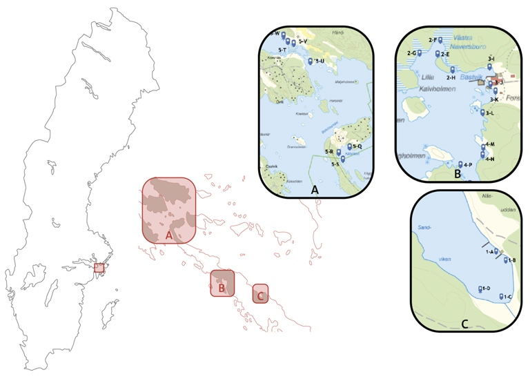
With Stockholm University’s research vessel Electra, they managed to obtain 10 cm diameter varved cores from eleven of the 13 selected coring sites in Kalmarsund, the strait between mainland Sweden and Öland. “Researchers working during the last century didn’t have access to offshore cores, but they have been key to integrating the varve chronologies in this difficult area. These offshore cores are an invaluable resource,” says Rachael Avery.
Faster off shore retreat rates
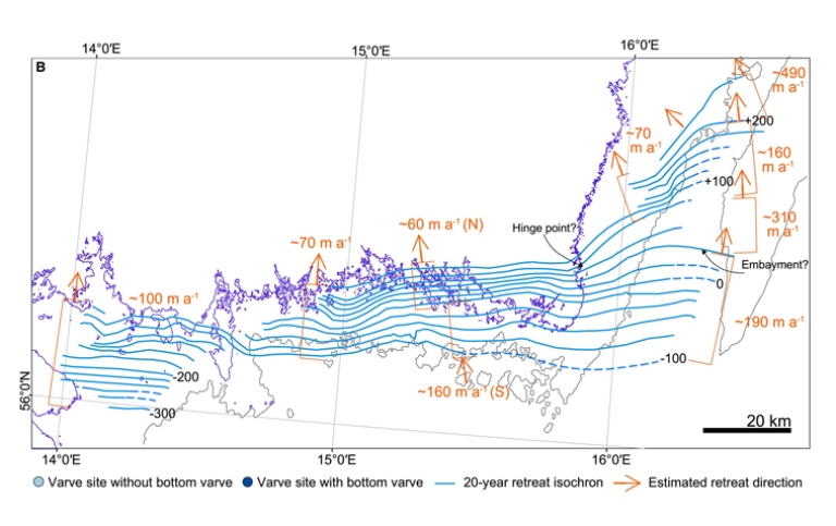
In the study, legacy varve records collected since the early 1900s also have been revisited, and combined with new terrestrial and offshore cores. The new chronology covers the subaqueous–terrestrial transition of the retreating ice sheet and spans 725 varve years of deglaciation. It reveals that the retreat rates in the offshore sector were three- to fivefold faster than where the margin was close to or above the palaeo-shoreline. This means a retreat rate of 160–490 meters per year offshore, compared to 60–100 meters per year onshore. The results are shown in the figure.
What are the practical implications of the results? Are they used to improve climate models?
“Most glaciers and ice sheets currently retreat at a breathtaking pace. But hardly any of our current Climate or Earth System Models are ready to interactively simulate the shrinking of ice sheets. In addition to several numerical challenges, we lack detailed observational knowledge to tune and test ice sheet models. The 725 years of annually resolved data is really unique as it allows us to verify changes in retreat rates dependent on zonal versus lateral retreat across an offshore versus onshore interface. The Department of Geological Sciences is currently adding an ice sheet modeller to our team, and we’re about to complete a high-resolution climate simulation for 15,000 years ago to provide the atmospheric forcing”, says Frederik Schenk, co-author of the study and leader of Research area 5.
Faster offshore retreat rates
The ‘father of the field’ of clay varve chronology was Gerard De Geer, a professor of Geology, and later also president at Stockholm University. Some of his original data was used in this new study. The pioneering work of De Geer can be seen on the Department of Physical Geography’s website (in Swedish). The continuation of De Geer’s work was carried on by new generations of scientists, including Lars Brunnberg and Barbara Wohlfarth and forms an important part of the legacy and work done at Stockholm University.
View data in the Bolin centre database:
bolin.su.se/data/hang-2021
bolin.su.se/data/avery-2020
The article "A 725-year integrated offshore terrestrial varve chronology for southeastern Sweden suggests rapid ice retreat ~15 ka BP" was published in Boreas on 17 November 2020. The article can be accessed here:
The study was financed by Knut and Alice Wallenberg foundation, Stockholm University and Bolin Centre for Climate Research, (RA5).
RA6 | Research highlights
What can we learn from mass extinction events in the past?
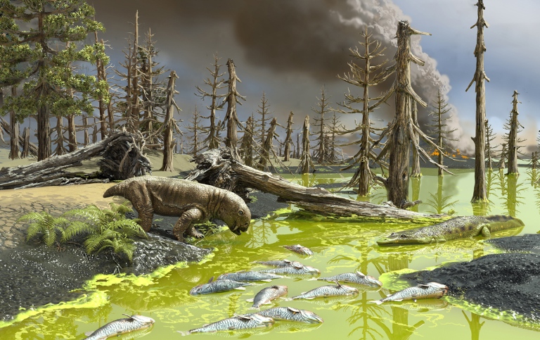
When looking back into the deep history of the Earth, there are signs of at least 13 mass extinction events of varying severity. The worst of them was the so-called end-Permian event 252.2 million years ago, when life nearly died out. A team of Bolin Centre researchers and colleagues investigated fossil, sedimentary and geochemical data from Australia to piece together the change in environmental conditions at that time, and how these relate to the climate changes we see today.
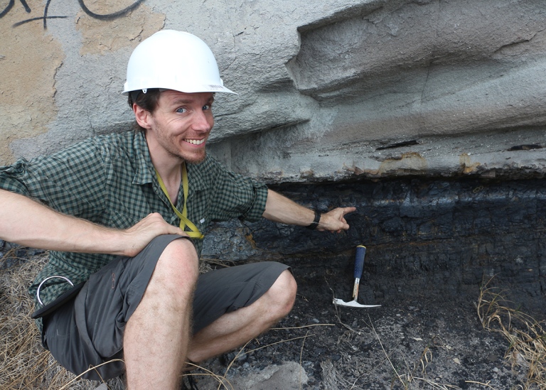
The world at the time of the Permian geological period was constituted by one connected landmass, the supercontinent Pangaea. After millions of years of a relatively stable global greenhouse, the environmental conditions changed drastically, caused by a volcano-driven hothouse climate. In a recent study, the researchers used organic microfossil and geochemical data from five stratigraphic sections in the Sydney Basin and they found a series of successive ecological phases in connection to the end-Permian event (EPE).
Pre-EPE: Late Permian wetland communities and ecosystem collapse
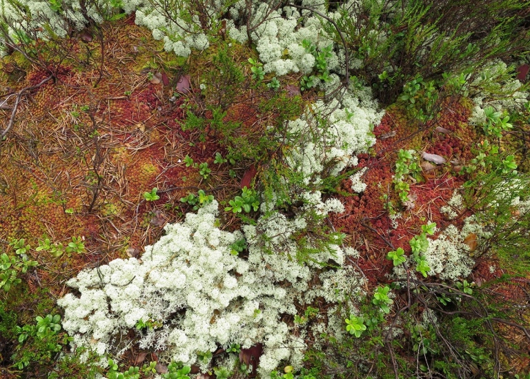
This phase, immediately before the end-Permian Event (252.2 million years ago), is represented in the fossil record by abundant wood, leaves and pollen typical of a flourishing wetland ecosystem. Algal diversity was relatively high, but their concentrations were low. Highly productive forest-mire ecosystems dominated the humid coastal plains of the Sydney Basin.
Early Post-EPE: The microbial rising from the “dead zone”
This 700,000-year-long interval initiated with sedimentary rocks typical of shallow standing water and fossils of fungi, charcoal and other opaque wood fragments. This picture corresponds to the earlier reported “dead zone”, characterized by widespread wildfires and deforestation which led to ponding and submerging of the land. The research team’s high-resolution analysis revealed successive green algal associations as the first colonizers of continental waterways following the “dead zone”. After this, recurrent toxic algal blooms occurred across the entire basin throughout the first 100,000 years following the EPE. One of the sites revealed fresh to brackish water conditions in which algae and bacteria reached extremely high concentrations. These values correspond to blooms of chlorophyte algae in lake sediments today, following local deforestation and the resultant influx of nutrients. At such high concentrations, these algae and bacteria lead to poorly-oxygenated waters upon their death, and many produce metabolic by-products that are toxic to animals. The researchers write: “Enhanced weathering intensity and destabilization of soils following deforestation, promoted nutrient influx into the floodbasins. Combined with elevated CO2, temperature and precipitation seasonality, these factors promoted numerous intermittent pulses of algal and bacterial proliferation.”
Late post-EPE: a recurrent microbial haven in the Early Triassic lowlands
Bacterial and algae continued to thrive throughout most of this 2.2-million-year-long interval, promoted by high global CO2 and temperatures because of continued volcanic outgassing. Large parts of the Pangaea supercontinent experienced strongly seasonal precipitation, and the regular drying prevented the establishment of permanent wetland floras, delaying the return of peat-mire carbon sinks. The researchers write: “Compared to pre-EPE wetland floras, the open post-EPE vegetation would have had relatively low biomass and evaporation rates, facilitating seasonally high water tables and maximizing light availability to aquatic bacteria and algae.” The combined data show that the conditions tended to promote enduring fresh/brackish-water ecosystems with sustained abundances of algae and bacteria within fluctuating coastal plain waterbodies.
The end of the microbial regime
It wasn’t until approximately 3 million years after the EPE that pre-extinction conditions began to return. This phase started 249.2 million years ago, and is reflected by increased abundances of land plant fossils, and a reduction of microbe-derived organic remains. This is in line with global vegetation trends, which are characterized by the widespread emergence of a new flora dominated by gymnosperms (flowerless plants that produce cones and seeds), promoted by climatic cooling.
How do the findings in the four phases relate to the climate change we see today? What implications does it have on our environmental condition?
“Today, humans are providing the ingredients for toxic microbial blooms in generous amounts, and with predictable results. When such bloom events occur in lakes and coastal environments, these cause animals to die en masse with devastating impacts on fisheries, severe health effects on humans and livestock, and an annual global economic cost of >$8B USD,” says Chris Mays, lead author of the article. He continues:
“This is a good example of what we can learn about climate change from the deep past. When life on Earth nearly died out, lethal concentrations of bacteria and algae choked the freshwater ecosystems, fed by extreme CO2, warming and soil nutrient run-off. All three of these ingredients are on the rise today, and the resultant blooms are leading to ecological stress that rivals the most extreme mass extinctions of the deep past.”
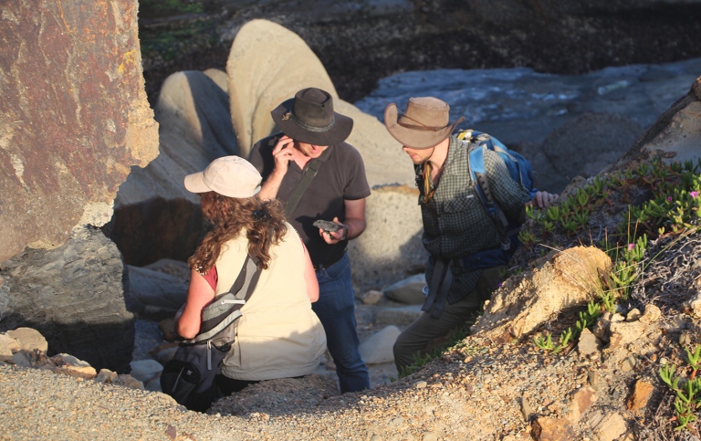
The study was conducted by Bolin Centre members Chris Mays, Stephen McLoughlin, Sam M. Slater, and Vivi Vajda, all affiliated with the Swedish Museum of Natural History, and colleagues Profs Tracy Frank and Christopher Fielding at the University of Connecticut, USA.
The article Lethal microbial blooms delayed freshwater ecosystem recovery following the end-Permian extinction was first published on 17 September, 2021, in Nature Communications. The article can be accessed here:
Lethal microbial blooms delayed freshwater ecosystem recovery following the end-Permian extinction
This work was funded by the Swedish Research Council (SE), the National Science Foundation (USA), and the Bolin Centre for Climate Research, (RA6).
RA7 | Research highlights
Forest management can both warm and cool understory plant communities
With climate change, it is generally expected that plants and animals move northwards, following their temperature preferences. But, on a hot summer day, a dense forest canopy and sheltering topography can create microclimates that are several degrees colder inside the forest than outside it. The capacity to reduce temperature extremes, means that forests can act as microrefugia for plants and animals in landscapes that otherwise would have unfavourable regional climate conditions. A team of Bolin Centre researchers has studied how forest management and climate impact plant communities at the local scale using data from the National Forest Inventory of Sweden. As forest density had a large effect on the temperature preferences of the plant communities, creating and keeping denser forests might be a way to counterbalance the climate effect on larger scales for understory plant communities.
The understorey is the space between the forest canopy and the forest floor at the ground level. Here, we find plant communities that have adjusted to, and prefer, specific temperature conditions. If it gets warmer, some of the species might go locally extinct, whereas other species might colonize new spaces.
The local climate in forest understories can differ substantially compared to outside the forest. A dense forest canopy and sheltering topography can create microclimates that are several degrees colder in the forest than outside it, which affects the composition of the plant communities in the understories. Another factor that influence the plant communities, is that forest structures often are characterized by cyclic changes driven by management activities, such as clear-cutting, subsequent planting and thinning. Changes in forest structure affect the capacity of the forest to buffer temperatures, and thereby change the temperatures experienced by the understory plant communities. In order to understand how and why understorey plant communities change in a climate context, there is therefore a need to consider both regional climate change and how forest density and structure varies over time.
In a study conducted in 2021, a research team used inventories from 11,436 productive forest sites in Sweden from the National Forest Inventory, repeated every 10th year between 1993–2017, to examine how the variation in forest structure over time influenced the temperature preferences of the plant communities. As a summarizing indicator of the plant community composition and to relate changes in community composition directly to temperature, the researchers used the Community Temperature Index (CTI), which is the average temperature preference of the species in a community. In other words, CTI is a metric that reflects the composition of warm- and cold-favoured species in a community. It is therefore expected to change with a changing climate.
With CTI data from the inventories, 2–3 times for each site, the research team evaluated to what extent the difference in CTI value between two inventories was related to two main factors: changes in forest density and changes in the macroclimate.
They found that the CTI values of the understorey plant communities increased after clear-cutting, and decreased during periods when the forest grew denser. In other words, cold-favoured species went locally extinct and got replaced with relatively warm-favoured species after clear-cut, whereas cold-favoured species colonized the forest again when it grew denser.
Importantly, the change in understorey CTI over 10-year periods was explained more by changes in forest density, than by changes in macroclimate.
Ditte Marie Christiansen is the main author of the study. What does these result mean?
“Our results show that changes in forest structures, in Sweden mainly by management activities, have a large role in explaining temperature preferences of species in understory communities, and that the impact from forest management is at least on short to intermediate time scales, larger than those from regional climate changes. This has two important implications. First, as forest structure is a main driver of plant community compositions regarding temperature preferences, we need to account for changes in forest structures when analyzing community responses to climate changes. Second, as temperature preferences of understory communities decrease with increasing forest density, we might be able to mitigate some effects of ongoing climate changes in forests by creating dense forest stands. However, under current management regimes in Sweden with thinning and especially clear-cutting, the mitigating effect is temporary.”
How will you continue with your findings?
“This article is part of my PhD thesis with the overarching aim to examine the impact of forest microclimate and its dynamics on understory plant species distributions as well as individual species performance. This study found large effects of forest management activities on whole communities, and my other projects focus more on individual species and their performance under different microclimate conditions. My main conclusion in my thesis so far is that microclimate matters and that we therefore need to take microclimate differences across the landscape into account when analyzing how forest plant species respond to climate change.”
The article Changes in forest structure drive temperature preferences of boreal understorey plant communities was published in Journal of Ecology on 9 December, 2021. The article can be accessed here:
Changes in forest structure drive temperature preferences of boreal understorey plant communities
RA8 | Research highlights
Predictive models of insects and the effect from climate change
With a changing climate, predictive ecological modelling becomes important. In the sphere of insects, climate warming is linked to macroecological shifts, such as range margin expansion, which can cause insects-related ecosystem disturbances. Bolin Centre researcher Loke von Schmalensee and colleagues set up an experiment to investigate what is required to predict insect development times in nature.
Many ecological processes are dependent on the temperature and how it varies. But predicting the temperature responses of organisms in nature is hard, and requires an understanding of how an organism’s traits respond to a range of temperatures they experience throughout their life cycle.
Ectotherms are organism in which the inner physiological heat sources are generally too weak to control the body temperature. For most of them, constant body temperatures are unnatural – their internal temperatures fluctuate with the surrounding climate. Yet, when estimating temperature dependent trait performance, for example growth and development rate, constant temperatures are commonly used. Now, an unanswered question is whether predictive models developed under constant temperatures leads to correct predictions in nature. It is known that certain mechanisms can kick in and cause differences under constant and fluctuating temperatures, such as acclimation or accumulation of thermal damage (potentially followed by repair during favourable temperatures). These mechanisms can lead to temperature-induced changes in thermal reactions, which makes it hard to bridge the gap between thermal performance under constant and under fluctuating conditions.
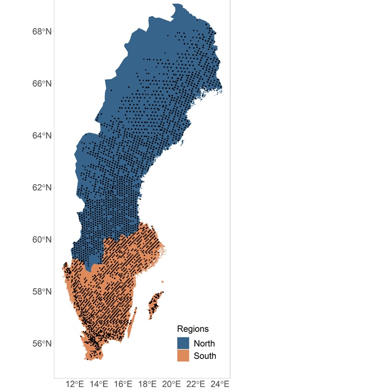
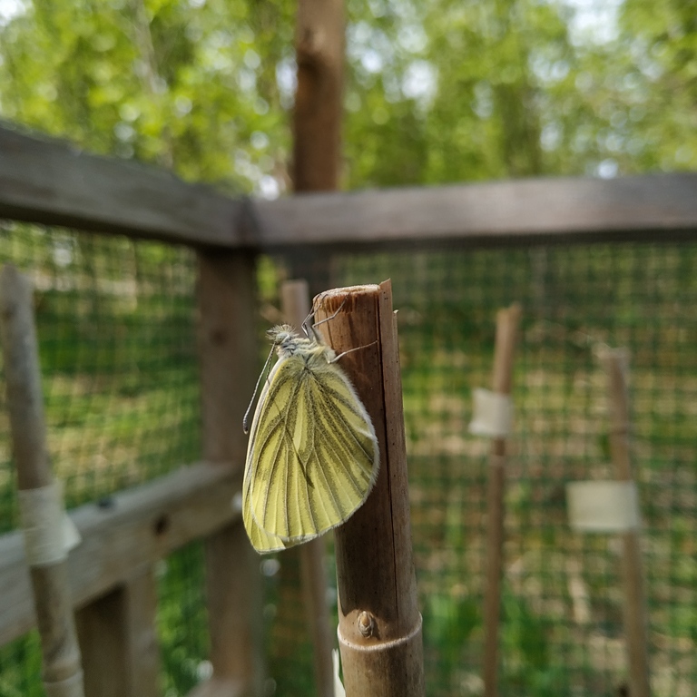
Bolin-researcher Loke von Schmalensee and colleagues set out to study this problem. They designed an experiment to measure the development rate of the butterfly Pieris napi under different conditions. Specifically, they wanted to know how the outcome of different prediction models with varying complexity and resolution of input climate data corresponded to the development rates on nine different sites across a heterogenous field area in Södermanland, Sweden. The time-span across two life stages, eggs and larvae, was measured in order to validate the models. In the field experiment, five containers were placed in a cage in each site, with coarse-meshed netting protecting against potential predators, while allowing for wind and rain to pass through. Temperatures were logged every 15 minutes at each site.
The prediction models were parameterized using thermal performance of Pieris napi in a laboratory environment. The individuals were treated at eight constant temperatures, extended over 10–35°C. Using the resulting thermal reaction norm, they could calculate expected development rates under fluctuating temperatures. They also measured the predictive impact from a low (means over 24 hours) to a high (every 15 minutes) temperature sampling frequency. By also incorporating data from a weather station in the nearby area of the field experiment, they could see how using macroclimate and microclimate temperature measurements influenced the results of the predictive model.
When comparing the results, they found that the development rate in the field can be predicted accurately across naturally variable microclimates under certain conditions, namely when using input temperatures measured frequently at organism-relevant scales together with well-estimated thermal reaction norms. Through an extensive collection of published data, they also showed that these findings are likely generalizable across insect taxa.
What practical implications does these results have?
“I think the findings are both relieving and burdening to people working with insect phenology (relating to seasonal timing) models. The fact that there seems to be negligible temperature-historic effects on insect development rates means that making accurate predictions in naturally fluctuating environments is actually feasible. Great news! On the other hand, our findings highlight that, in order to do so, one must pour a lot of effort into the methodology. Thankfully, microclimate modelling and monitoring are advancing and becoming increasingly available tools to biologists,” says Loke von Schmalensee.

What would be the next natural research in this research area?
“The natural step is to start looking at other environmental variables. For example, how does host plant quality influence development rates under variable conditions? Can we find any general patterns? In order to build more complete models of insect population dynamics, there are many life history traits to consider. Sure, being able to ignore temperature-historic effects on development rates removes a dimension and greatly reduces complexity in such a model, but there is still much we don’t know about how insect populations behave in nature.”
The article Thermal performance under constant temperatures can accurately predict insect development times across naturally variable microclimates was first published on 25 May 2021 in Ecology Letters. The article can be accessed here:
This study was made possible through funding from the Bolin Centre for Climate Research, and is a part of the Bolin Centre Research Area 8, research in biodiversity and climate.
Last updated: October 8, 2023
Source: Bolin Centre for Climate Research